As humans expanded out of Africa into the rest of the world, they adapted to a whole host of new habitats, pathogens, and food sources. In recent years, there has been an explosion of interest in identifying the specific genetic loci underlying these adaptations using whole genome genotyping (and now sequencing). In this post, I’ll outline some of the basic principles of how these methods work.
Actually, I say “basic principles”, but what I mean is “basic principle”, because there’s only one: every method for detecting positive selection tries to identify alleles which have gone up in frequency unusually fast. The differences between methods for detecting selection all lie in the information they use to find such alleles (since for the moment, we don’t have good data on historical allele frequencies).
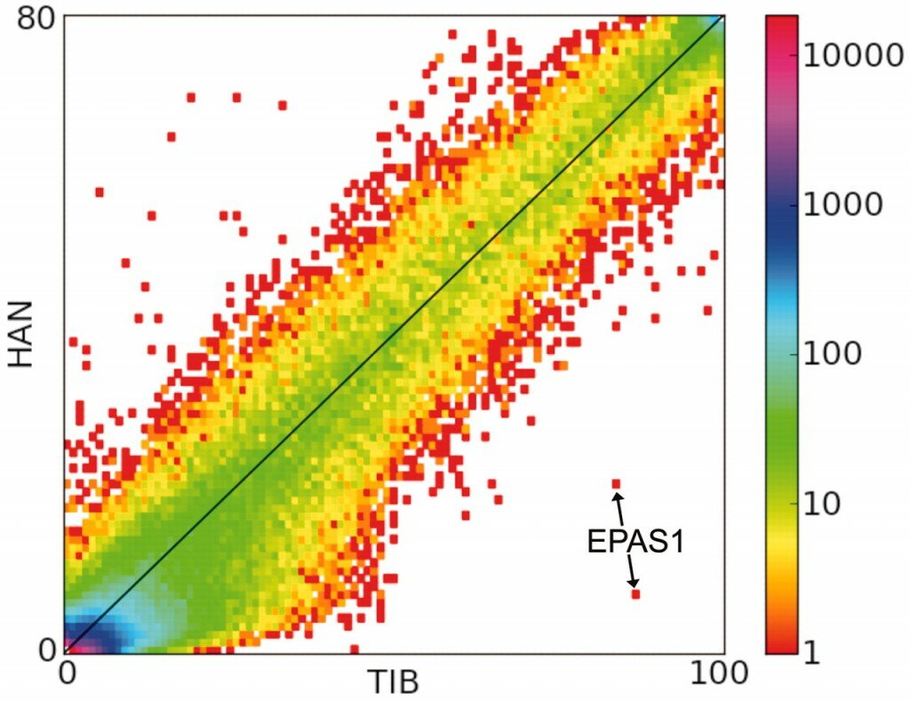
One class of methods makes a straightforward assumption: imagine that selection is acting in one population, but not another. In this case, the allele frequencies of the selected alleles in the first population will go up relatively quickly compared to the frequencies of those same alleles in the second population. The test, then, is simple: are there alleles that have unusually large allele frequency differences between two populations? This principle was recently used to identify the gene EPAS1 as potentially important in adaptation to high altitude in Tibetans [1]. On the right is the relevant figure from that paper: a two-dimensional histogram of allele frequencies in a Han Chinese population (HAN) versus those in a Tibetan population (TIB). The points labeled EPAS1 are clear outliers in this distribution.
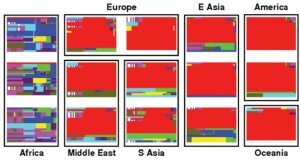
Another class of methods makes a different (and perhaps more restrictive) assumption: imagine that selection is acting on a mutation which is new (or at very low frequency) in a population. Again, selection will act to increase the frequency of the allele, with the result that there will be a young allele at relatively high frequency in the population. The age of an allele can be assessed by measuring the amount of genetic variation around the allele (as time passes, more mutations occur in the region) or the length of the haplotypes on which the allele sits (as time passes, recombination breaks up the association of the allele with nearby ones). Again the test is clear: find the young alleles at unusually high frequency. As an example of this, consider the genetic variation around the pigmentation gene KITLG pictured on the right (from [2]): each plot represents a population, each horizontal line in the plot represents a 500 kb haplotype in the population, and identical haplotypes are the same color. In the non-African populations, you can clearly see the large blocks of red, indicating that there is a long haplotype with very little variation (ie. a relatively young allele) nearly at fixation in these populations. Indeed, this gene is known to contribute to lighter skin in non-African populations [3].
I’ve tried to avoid the alphabet soup of acronyms for tests for selection in the above discussion, but people who have read papers using these tests will recognize tests based on haplotype homozygosity or the site frequency spectrum as tests of the latter type, and tests based on FST as tests of the first type (there are also tests like XP-EHH which combine aspects of the two). Though all these sorts of statistics have their pluses and minuses (perhaps to be discussed in future posts), the general principle remains quite similar.
[1] Yi et al. (2010) Sequencing of 50 Human Exomes Reveals Adaptation to High Altitude. Science. DOI: 10.1126/science.1190371
[2] Coop et al. (2009) The Role of Geography in Human Adaptation. PLoS Genetics. DOI:10.1371/journal.pgen.1000500
[3] Miller et al. (2007) cis-Regulatory changes in Kit ligand expression and parallel evolution of pigmentation in sticklebacks and humans. Cell. DOI:10.1016/j.cell.2007.10.055


 RSS
RSS Twitter
I liked very much this introductory post. It seems to me that the first method is highly similar to those used in genome-wide association studies for the discovery of SNPs associated with a disease, but in this case you compare two populations instead of one case group and one control group. Am I correct?
Moreno,
This first approach is similar to a genome-wide association study to a certain extent. However, there’s a major difference:
In a standard, well-designed GWAS, the only reason the cases and controls differ in allele frequency is if an allele contributes to diseases risk (to an approximation). So any small difference in allele frequency, if reliable, is interesting.
By contrast, two populations differ in allele frequency due to genetic drift as well as natural selection. So the null hypothesis is not that the two populations have identical allele frequencies, but rather that the difference in allele frequencies is lager than you would expect due to drift. This is a much more difficult thing to quantify (since it depends the generally unknown demographic histories of the populations), so what people generally look for are major outliers, rather than doing formal tests for association.
Thanks for the clear explanation, so in this case we look for extreme situations. Thank you!
The work by my colleague Bob Moyzis and his group for the 48-bp VNTR in the dopamine receptor D4 (DRD4) gene (see Ding et al, 2002, PNAS, v 99, p 309-314) and the linkage disequilibrium decay test (see Wang et al, 2006, PNAS, v 103, p 135-140) are excellent examples of recent positive selection. A lecture on YouTube by Moyzis (http://www.youtube.com/watch?v=zbyaryb9AeQ) is worth watching.
Thanks James. For those interested, the LDD test referred to is of the second type discussed in the post (ie. it looks for young alleles at high frequency).
Great review post Joe. One thing that I couldn’t understand about the EPAS1 variants in the first paper you cite is why there isn’t a small Gaussian of variants surrounding those two markers in the plot; in the same way that we see residual LD around a significant hit in a Manhattan plot. Were this a Manhattan plot, I would be suspicious of those sites being artifact, why is that not the case here? Could it have something to do with the fact that this was an exome study but that EPAS1 variants were both intronic (but still typed, fortuitously)?
That’s a good point. I think the answer is that, since this study was done by exome sequencing, there simply aren’t a lot of typed variants in LD with the ones identified. That is, there probably are quite a few things in LD (you can see that in another paper on the same subject), but since exons are tiny compared to introns, most weren’t genotyped by their approach.